Teaching a World Model to Play Pokemon

I think some of the most fascinating work happening in the field of Artificial Intelligence surrounds world models. There are many kinds of world models (and the term itself has become a bit overloaded), but one of the most exciting architectures for world models is Yann LeCun’s JEPA (Joint Embedding Predictive Architecture). There are many variants, and one that caught my eye in particular was LeWorldModel1. It seemed small enough to train locally on my RTX 3080 Ti and had a simpler design than many of the previous JEPA architectures.

Pokémon Red is a game where you explore a world, collect creatures called Pokémon, and use them in battles.

You use the direction buttons to walk around or move through menus. The A button interacts with things, advances dialogue, and confirms choices; the B button usually cancels or backs out. Choosing a starter means approaching a Poké Ball (a container that holds Pokémon) and getting through the dialogue that confirms your choice.

Near the beginning of the game, the player is inside Professor Oak’s lab, where he offers you your first Pokémon: Bulbasaur, Charmander, or Squirtle. These are the three “starters,” each waiting in a Poké Ball on a table in his lab.

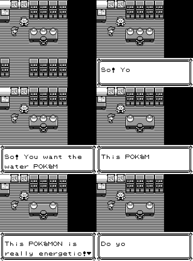
The GIF above is the final result of the model training: the model planned a sequence of button presses that selected Squirtle. There were more difficulties and setbacks than I expected, even though the model had looked promising in simpler tests.

The goal was relatively straightforward: defeat Professor Oak’s grandson. Breaking it down into multiple steps, I came up with:

It quickly came to my attention that this might be ambitious for a first experiment–so I narrowed it down to selecting a starter from a saved state in Oak’s Lab, where acquiring any of the three starters would count as a successful attempt.

From the saved position in the lab, having the model press A twelve times is enough. But can the model learn that? The model could also just wander around aimlessly, maybe in perpetual torment inside Oak’s lab. Or the model could press B after every few sequences of A, cancelling its effort when it almost reached its goal.

A world model is a model in which we begin with some current state or observation, and some action happens that modifies this state, producing a new observation. Realistically, there should be some sort of correlation or hopefully causation between the action on some state and the new state it produces. The goal of the world model is to learn this correlation. Let’s say the current observation is a screenshot of Professor Oak’s lab, with the player in front of the Poké Balls, and the action is pressing left, moving the player one tile to the left–producing the new end screenshot. The goal would be for the world model to develop some form of intuition that pressing left moves the player left.

Here (o_t) is the current screenshot, (a_t) is the button pressed, and (F) is the function the world model learns to predict the next screenshot (o_{t+1}).

But the goal should be to generalize–the model shouldn’t learn that pressing left in Professor Oak’s lab moves the player left, but that pressing left anywhere should move the player to the left.3

As an aside, this setup might sound somewhat similar to reinforcement learning. But crucially, the world model learns to understand the state dynamics without a reward, aka being reward-free (more on this later).

So if what we are really interested in is the state-transitions and the dynamics of the environment4 and all we have are observations (in this case, in the form of screenshots from our game), does the model learn to predict screenshots?

No, what the model actually learns is to predict within its latent space, also known as its embedding space. We first need to take an encoder that, when given a screenshot, produces an embedding.

An embedding is a learned representation of an input as a vector of numbers. An encoder can turn an image, a sentence, or a sound into such a vector, giving another model something it can compare, predict, or use as input.

The entries are not hand-labeled features: one coordinate does not have to mean “color” or “position.” Information can be spread across many entries, and some details of the original input can disappear altogether. Whether an embedding is useful depends on which distinctions the encoder learns to keep.

With the embedding representing the current observation (o_t), we can then have a predictor model that, given an action (a_t), tries to predict the future embedding. With this future predicted embedding, we can try to compare it to the real embedding produced by the future observation (o_{t+1}). This is actually rather simple: just pass the new screenshot through the same encoder and we get the real future embedding. The goal is then to just have:

Here, (\hat z_{t+1}) is the predicted next embedding, and (z_{t+1}) is the embedding of the screenshot that actually followed.

Press APredictorPredicted embeddingMSECurrent embeddingTarget embeddingSame weightsEncoderEncoderCurrent screenshotNext screenshotWriting this out for one step:

Here, (x_t) is the current screenshot, (a_t) is the action, and (E) and (P) are the encoder and predictor. Importantly, the predicted embedding (\hat z_{t+1}) is never turned into a screenshot, and we can compare it directly with (z_{t+1}).

To learn the difference between our prediction and the ground-truth embedding, we will use the ol’ reliable loss function Mean-Squared Error.

It looks kind of complicated but you can imagine it as just a distance function. We are basically just trying to measure the distance between our two embedding vectors.

Everything seems simple enough: minimize this function–we have a world model that can play Pokémon, right?

But it’s never so simple, and there is actually a dangerous degenerate case that can happen. Remember that we are training the encoder and the predictor, and the encoder appears twice in each training example:

In the worst case, the encoder starts to learn to embed every screenshot as the same embedding (c). Then, the predictor also begins to learn to predict that the next embedding will be (c). This is called latent collapse and means that the model has found a trivial way to reduce the loss function–by collapsing all embeddings to the same embedding.

So the prediction loss can be minimized by putting every screenshot into the same point. If we could somehow keep the embeddings from collapsing to the same point, then we can get back on track at producing a useful world model. This is the perpetual problem of JEPA, and many different JEPA model architectures have come up with different ways to try to prevent latent collapse.

One possible fix is to make sure each number in an embedding changes across screenshots. But we have to be careful about how the embeddings spread out. Imagine embeddings with just two numbers: ((1,1)), ((2,2)), and ((3,3)). Both numbers change, but the second always copies the first. The points form a line, which only means it has one dimension of data instead of spreading over a two-dimensional area. With 192 numbers, the same kind of redundancy is harder to notice.

The LeWorldModel paper chooses a relatively simple solution–at least compared to many of the other JEPA architectures–called SIGReg, or Sketched Isotropic Gaussian Regularization.

SIGReg asks for a stronger shape. Across a batch of screenshots, it encourages the embeddings to resemble a standard isotropic Gaussian:

The isotropic Gaussian has a mean of 0, and the identity matrix (I_D) as its covariance matrix. In two dimensions, that is a round cloud rather than a point or a line. You can see here that the isotropic Gaussian forms this more evenly spread out shape in all directions:

Enable JavaScript for interactive controls.

Suppose the encoder produces a batch of embeddings (z_1,\ldots,z_N\in\mathbb R^D) which form a cloud like in the above figure. SIGReg picks a random direction (u) of length one and measures where each embedding falls along it:

The (h_i) are now ordinary numbers instead of (D)-dimensional vectors. If the original cloud really followed (\mathcal N(0,I_D)), the numbers along any unit direction would follow (\mathcal N(0,1)).

In two dimensions, let a random embedding be (X=(X_1,X_2)), where (X_1) and (X_2) are independent standard Gaussians. Choose the unit direction (u=(3/5,4/5)). Its projection is

A weighted sum of independent Gaussians is still Gaussian, and its mean is zero. To find its variance, remember that variance averages squared deviations from the mean. Multiplying (X_1) by (3/5) therefore multiplies its variance by ((3/5)^2); the same applies to (X_2). The mixed term averages to zero because the coordinates are independent and centered at zero, so their variance contributions add:

The same argument works in (D) dimensions. For any unit direction (u=(u_1,\ldots,u_D)), its squared components add to one: (\sum_j u_j^2=1). The projection (u^\top X=\sum_j u_jX_j) is Gaussian with mean zero and variance (\sum_j u_j^2=1), so it follows (\mathcal N(0,1)). In compact matrix notation, that variance calculation is (u^\top I_Du=|u|^2=1).

The problem has become a one-dimensional question: do these projected numbers look like samples from a standard Gaussian?

SIGReg answers this with a characteristic-function test.

A characteristic function is another way to describe the shape of a probability distribution.

For a random vector (X), it is defined as

You can think of (t) as choosing a direction and a scale at which to “probe” the distribution. The characteristic function tells us what the distribution looks like under that probe.

Notice that this only depends on (|t|), the length of (t), and not the direction it points. That matches the intuition behind an isotropic Gaussian: it looks the same in every direction.

The value of the characteristic function is that it is unique to each probability distribution, and therefore if you can show that a random variable’s characteristic function matches another random variable’s everywhere, then they have the same distribution.

For each direction, SIGReg compares the characteristic function estimated from the projected samples with the known one for (\mathcal N(0,1)). We then use the Epps–Pulley test to turn the mismatch into a penalty. You can find more details in the original LeJEPA paper or Appendix A of LeWorldModel.

We average that penalty over 1,024 random directions, then use its gradient to update the encoder. The finite set of directions is then used as an approximation to checking the full distribution.

The final training objective function looks like this:

Here, the 0.1 controls how much the regularizer contributes to our training by discouraging the erasure of variations among screenshots.

We now have a way to train a model from pairs of screenshots and actions. Where do those pairs come from? I recorded 42,382 grayscale frames from the Pokémon Red emulator, grouped into 1,009 short trajectories. Some trajectories follow scripted routes to a starter. Others add noisy actions to those routes, or move around more randomly. For each step, the recording contains the current frame, the button pressed, and the frame that followed.

It’s actually important to have the messy trajectories. A model trained only on the clean route might see A pressed whenever a dialogue box appears and never learn what B does there. The planner, however, is going to propose all sorts of button sequences, including bad ones, and it needs predictions for those sequences too. This does not make the dataset a complete map of Pokémon Red, but it gives the model more than a single demo