How Witten Used Quantum Field Theory to Understand Knots

Curt Jaimungal

Sep 25, 2026

36

9

6

Share

Witten published a paper in 1989 which helped secure him the Fields Medal the next year.

But saying “the Jones polynomial is a Wilson-loop expectation value” doesn’t explain anything if you have to Google every other word… And it doesn’t even do justice to the paper, regardless. Like, what’s the loop? Where does the field come from? And how does averaging over anything tell us about knots?

Curt’s note: Please try and view this on a desktop, and not mobile… There is in-line math that doesn’t get rendered on mobile for some reason, so this post won’t make as much sense.

I recall going through this paper when I was younger and being struck how my initial impression (that this was “tying knot theory to quantum theory”) was completely underselling what was done in just 40 or so pages. At first I was thinking, Witten connects the Jones polynomial to QFT. That’s outstanding itself. But then it just keeps going, man. Atiyah asked a question about 2D projections, which Witten answers. A few pages later you realize that it’s not even about knots (per se)!

Then you find out that Witten figures out that any 3-manifold gets new invariants of the manifold itself as a result of this! (this will be explained a bit more below). And then Witten shows that if you swap (\mathrm{SU}(2)) for (\mathrm{SU}(N)), you get a different polynomial than the Jones polynomial (something called the HOMFLY polynomial). Then you find out that (\mathrm{SO}(N)) gets you the Kauffman polynomial. And then Witten shows how all of this is tied to 2D conformal field theory with something called surgery theory, which is about cutting and joining different manifolds. And then there’s Erik Verlinde, who had a conjecture, and Witten gave a new proof of it in this paper itself. And then there’s something about “framing” that Witten uses to fix a phase, and where Ray-Singer torsion comes from, and he did all of this in just a single paper. Man, many of these would be one tenth of a career for most people, and he did it all in one single paper, not even in a single year. There’s more from this year, which I’ll probably cover later on the Substack.

I’m going to focus on just one tiny aspect of this 1989 paper and try to help you see why it was so inventive, surprising, applicable (physically), and genius. He found a new type of topological quantum field theory. A topological quantum field theory is a quantum field theory that doesn’t depend on the metric. Then you realize there are two ways that this could occur. One is if the metric indeed is present, but every physical answer turns out to not depend on it, then you’re in some sense independent of any given metric. Another way is that you don’t involve the metric to begin with. This is the route Witten takes here. Confusingly, the first kind is now called a TQFT of “Witten” type, whereas the other one is called Schwarz type (after Albert Schwarz, who built metric-free theories like this in the late 1970s).

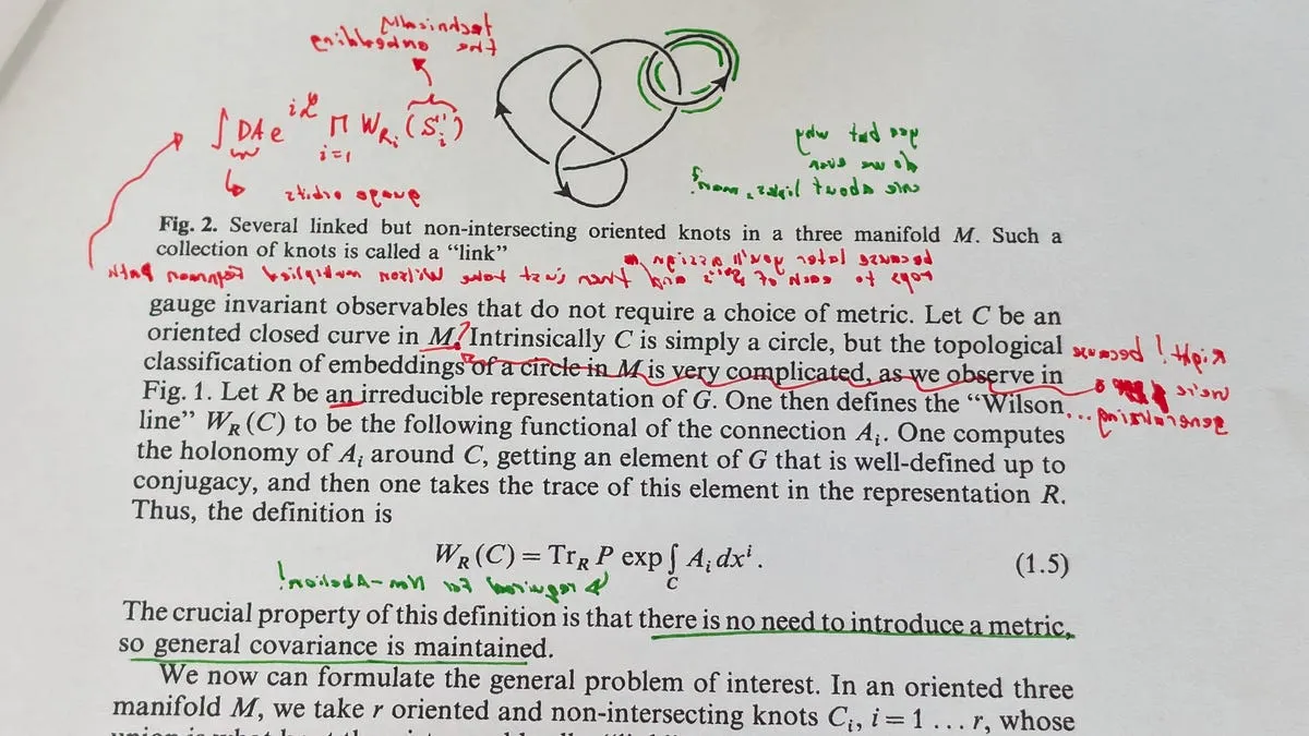
A mathematical knot is a closed, non-self-intersecting curve in three-dimensional space. You can bend or stretch it, but you can’t “cut it” or pass one strand through another. The best way to think about it is as the cicle ((S^1)) embedded in three dimensions (usually (S^3), the higher dimensional sphere than the one The Raptors are familiar with).

The unknot is a loop that can be deformed into a circle. A trefoil is the familiar three-crossing knot. Those crossings belong to a drawing: the actual strands pass above or below one another without touching.

NOTE: The types of knots you encounter in knot theory are not the kind of knots that you encounter in regular life. Regular life knots usually serve some purpose, such as anchoring a boat to something or tying your shoe lace together. The ends of most of what we colloquially call “knots” are actually cut and free to move around. Thus it’s more like an embedding of ([0,1]) into (\mathbb{R}^3). A mathematician’s knots are more like a horribly tangled rubber band, though even here, unless the rubber band was molested in some manner, they could all potentially (with great work) be made equivalent to the “unknot” (the trivial knot) and therefore not terribly interesting.

A knot invariant is something that gives the same answer to every (permitted) deformation of a knot. Length doesn’t’ qualify, since stretching changes length and stretching is permitted. Counting crossings in a particular drawing doesn’t qualify either.

Jones found an invariant called the Jones polynomial. You give this Jones-procedure a knot, and it outputs a finite expression in a variable, which is usuallye called (q). Negative powers are allowed, so the precise term is Laurent polynomial. This is a generalization of the ordinary “polynomial.” Actually, when you were in school learning about polynomials, perhaps the question occurred to you: “Why not allow negative numbers in the exponent?” To me, the Laurent polynomial has always been the more natural polynomial.

Anyways, in a convention I’ll retain throughout this Substack, one trefoil and the unknot give:

The above (V) is the Jones polynomial of said knot. If you allow (q = 2), then the trefoil gives (2 + 8 - 16 = -6). The unknot will equal (1). Thus, because their polynomials differ, the curves can’t be deformed into one another under our permitted rules. This is an example of a “topological invariant.”

Like most topological invariants, if you have something that differs between two spaces, then the two spaces are topologically inequivalent, however, if you calculate an invariant to be the same, then you may or may not be dealing with different spaces. The test at this latter point is “inconclusive.”

Witten sometimes called topological invariants “generally covariant” in his paper, but I won’t say that here because it could be slightly confusing. Just note that he uses those terms, in that 1989 paper, pretty much interchangeably.

So, if the original invariant of Jones already worked fine and was provably an invariant, what did Witten do? Well, Witten had a question in mind which came from watching a talk given by Michael Atiyah in 1987. It was about how to construct this invariant directly from a field theory on the three-dimensional space containing the knot. The first line in the Quantum Field Theory and the Jones Polynomial paper talks about his inspiration for the paper itself.

“Pick a knot. Any knot.” said the naughty magician.

“Keep that knot fixed, and look at every point in the surrounding space. Attach a copy of a two-component complex vector space.” said the unhirable magician.

An these vectors have entries (z_1) and (z_2).

Witten specifies how to “update” the vector when it’s moved along the knot. When I say “update,” what’s meant is that you have a 2-by-2 matrix that acts on the vector, along with properties of keeping the total length fixed, (|z_1|^2 + |z_2|^2), and also having determinant 1. The collection of these is the group (\mathrm{SU}(2)).

Witten chose this specific group (and its two-dimensional “irreducible” representation) because it turns out this is what gives you the ordinary Jones polynomial. Witten created (among other things) a procedure that takes in a group, and out pops an invariant. Other gauge groups or representations give related invariants. I mean, I remember reading this and being blown away even before I saw the proof. Just blown away at the conclusion that we’re going to lead to, almost like watching a cold open of Breaking Bad. You’re like “how? how did they get there? how did he (Witten) even think of that in the first place?”

So far, we haven’t introduced a physical particle moving around the knot, though its tempting to think of knot diagram as a spacetime trajectory diagram. The two complex entries don’t automatically make it a Weyl spinor. This is because the matrices act on an internal index, with no spacetime spinor transformation law specified.

The procedure Witten gives is one Wilson gives in his famous “Wilson loops.” That is, you divide your knot into lilliputian segments, and look at what happens to your tentative irrep (your two component vector) along the way. Think of it like if you’re running a marathon and there are various check points, and the first checkpoint person (is there such a thing?) say “hey, if your shirt is black I’m going to add a bit of color, and if it’s too colorful I’m going to dull it” and the next checkpoint person says “If you have no water in your hand I’ll give you some, if you do I’ll take yours away” etc. for each each checkpoint with more and more bizarre rules, so that each person gets transformed in some manner by the time they finish the race (provided the runner is not disconcerted by these procrustean checkpoint people).

Mathematically, suppose the first update is (U_1), the next is (U_2), and so forth. After the whole circuit, the combined update is:

Here (K) denotes our knot and (N) the number of segments. The earliest operation is on the right hand side because it’s what acts first on the vector (the runner, in the above odd example).

The following matrices both belong to (\mathrm{SU}(2)):

This means that the order of the application of the matrices/transformations/checkpoint-people-rules matters. This is the noncommutativity that has to be preserved as segments become arbitrarily diminutive (also known as non-abelian).

A connection, or gauge field, is what tells you which infinitesimal updates to apply at each point and in every direction. Call it (A). For a tiny displacement, its going to be basically the identity plus a little bit:

The identity matrix (I) leaves you unchanged. I removed a purely complex convention to make the above slightly more pedagogically clear. The index (\mu) usually spans four dimensions, but we’re dealing with knots, so it’s spanning over three directions. The last term collects corrections quadratic or higher in the displacement, and it’s what you ignore.

In this convention, each (A) component is anti-Hermitian: transposing it and complex-conjugating gives you back minus the original (A). It’s also traceless, meaning its diagonal entries sum to zero. Exponentiating the (A) times a real displacement (the dx’s) produces an (\mathrm{SU}(2)) matrix.

When you take the limit of the (ordered) product around the closed route of the knot, you get something called its holonomy:

The square brackets are there to remind you that the answer depends on the chosen connection / gauge field. The (P) means path ordering: that is, keep the sequence of matrix multiplications because as we mentioned before, the order matters since we’re dealing with non-commutative transformations. I added the complex factor (i) above to be consistent with the literature now, but nothing about my above explanation changes substantively. Pulling out that (i) makes A Hermitian.

We still have a matrix, though. To obtain a number, take its trace, the sum of its diagonal entries:

This is the Wilson loop in the two-dimensional irreducible representation. If you just have the identity, then the holonomy (Wilson loop) gives 2. The diagonal matrix (B) from mabove gives (i - i = 0). All of this is prior to anything “quantum.” It’s just classical so far. If you don’t know what I mean by quantum vs. classical, this will be explained shortly so hold on.

Allow me to pause on the question of “Why the trace?” The reason is that when you take the trace you make it independent from a basis, a value which is at the heart of differential geometry Specifically, you can the internal basis separately at every point and the changes at adjoining endpoints cancel (recall, it’s a loop where you start where you began). At the starting point, the holonomy transforms by conjugation, where (g) is the basis change there:

Conjugating a matrix leaves its trace unchanged. So, as you may know from libnear