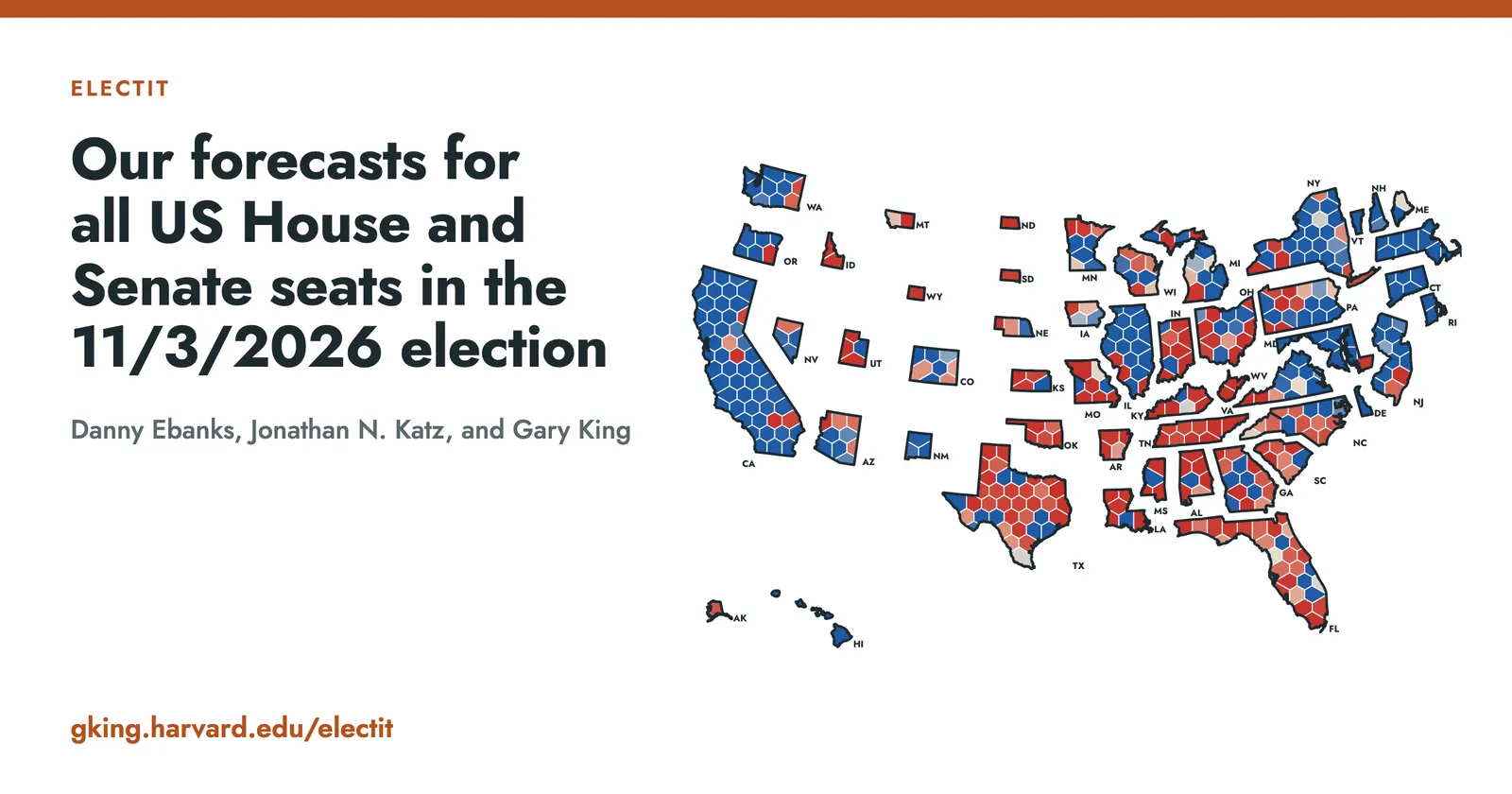
ElectIt: U.S. Elections Forecast

Our structural covariates, Xit, are the election's past results (its own lagged effective vote and the district's lagged presidential, Senate, and governor votes), incumbency, open seats left involuntarily or by a strategic exit, the South, an uncontested election, and a midterm penalty, which represents the strong tendency of the president's party to lose ground in midterm elections. Their slopes, 𝛽t, show parameter drift with coefficient stability: they vary a lot in the long run but change very little from year to year, so each follows a random walk, 𝛽tk ∼ N(𝛽t−2,k, 𝜎𝛽k2).

The candidate effects, 𝛾D(i,t) and 𝛾R(i,t), model candidate uniqueness. They are person-specific intercepts on the Democratic and Republican candidates in the election, drawn from a common distribution, 𝛾c ∼ N(0, 𝜎𝛾2). Each is the candidate's valence net of party, incumbency, the district's partisan lean, and the model's other systematic components, and an election in which one major party fields no candidate drops that party's term.

The national trend, 𝜂t, allows for positive cross-district covariances: it affects all districts in one election in roughly the same way, over and above the information in X. It models the familiar observation that some years are good for Democrats and others for Republicans, even if we do not know which is which ex ante: 𝜂t ∼ N(0, 𝜎𝜂,d(t)2), its standard deviation estimated for each redistricting decade, d(t). In midterm years, we also account for year-to-year variation in the midterm penalty, as the generic ballot provides information about both 𝜂t and the midterm penalty.

The error, 𝜔it, models district-level political surprises. We use the additive logistic Student t (ALT), which, unlike the normal, constrains the vote proportion to the (0,1) interval and has appropriately fatter tails to represent surprises, with more of its density concentrated near the mean. Its scale, 𝜙it, and degrees of freedom, 𝜈it, depend on Zit: an open-seat indicator, the marginal distance from 50/50 in the district's lagged presidential vote, and an indicator for single-district states and the Senate, with slopes 𝛿 and 𝜆, intercepts 𝜁 and 𝛼, and redistricting-decade effects 𝜁d and 𝛼d. Safe seats' future vote shares are relatively predictable from one election to the next, whereas a competitive seat exhibits a far greater tendency to surprise.

We formally distinguish between the observed vote, vit, and the effective vote, vit*, the vote proportion that would have been observed if the election had been contested. We estimate the unobserved effective votes as unknown parameters with all the others, under a censoring assumption: candidates running unopposed would have won even if the election were contested.

The forecast. Each of the 160,000 simulations draws the model's parameters from their posterior, then 2026's national trend, 𝜂, from N(0, 𝜎𝜂2) with the 2020s' 𝜎𝜂, then every election. With equal weights, the simulations are the Post-Nomination Forecast: an election's chance is the frequency with which the Democratic candidate wins in our simulations, and the chance of a Democratic House is the share in which Democrats win 218 or more seats.

Our model, LogisTiCC, simulates each House and Senate election times. As reported in our paper, we estimate a national trend, 𝜂, which shifts every election in a given year in logit space by the same magnitude. Model + Generic Ballot keeps every simulation and gives each one a weight. A simulation counts more when its national House vote agrees with the most recent observed value of the generic ballot. We build it in eight steps.

Compute each simulation's national vote. A simulation's national vote, V, the Democratic share of the two-party House vote, is:

Here i is a district, and ci is election i's logit without the national trend: its fundamentals, its candidates, and its surprise. The inverse logit, logit−1(x) = 1/(1 + e−x), turns a logit back into a share. To replicate the official count of the popular House vote, our estimated national vote is weighted by how many votes we expect to see in each district, which we measure by Ti, its share of 's presidential turnout, with each unopposed seat at its recorded share. In the unopposed elections of 1946–2024, the official count recorded 66% as many votes for their turnout as in contested elections (33% in Florida, which recorded no votes for half of them, and 81% in California). We estimate turnout based on current district lines, calculated using precincts from 2014–2024, and county-level returns from 1946–2012. Ti is not a known parameter: it is a forecast, and the House electorate it stands in for changes from year to year. So we add one-step-ahead forecast noise to it (step 5), estimated from all election results prior to the forecasted year: now points of the national vote.

Incorporate a tied-election baseline. To allow for more effective simulations in the Build Your Own modeling feature, we augment the tails of the prior distribution (our LogisTiCC forecast). We shift each simulation's national trend by Δ = , toward the . This shift makes Democrats win 218 or more seats in exactly half of the set of effective simulations. We call this set of simulations the Tied House Election Baseline, and their average national vote is %. This allows us to explore parts of the simulation space far away from what the model expects after the primary. This is especially helpful if there are large shifts in the fundamentals over the course of the campaign. We then sample from the mixture of these two normal distributions:

Here 𝜎𝜂 is the model's standard deviation for the national trend. The mixture only supplies draws. Step 7 counts each draw by the model's own prior for 𝜂, so if the generic ballot holds no useful information, the forecast returns to the Post-Nomination Forecast.

Fit a regression line that predicts the generic ballot from the national vote. We fit a regression of the generic ballot on the official national vote, using . For previous forecasts, we only use data available prior to that specific election. We use the final generic-ballot margin, G, and the national House vote, V.

Here a is the intercept, b is the slope on the logit of V, and e is the poll's error, with standard deviation 𝜎G. We estimate the regression line by weighted least squares:

National polling errors have decreased since the , so we allow the size of errors to drift over time, from in the to in the . For each holdout forecast prior to 2026, we estimate this regression for midterms and presidential elections separately. We only estimate the national vote once we have at least 5 years' worth of data points in each regression. Since we do not observe 5 midterm and 5 presidential elections prior to 1958, we pool both midterms and presidential elections together to estimate the above regression (as we have generic ballot estimates going back to 1938) for 1948–1956.

Polls have become more accurate, so we count recent midterms more, at nine possible rates, 𝜆, from 1 (all midterms count the same) to 0.5. We weight each rate by how well it predicted the generic ballot in each earlier midterm, using only the elections before that midterm. .

Steps 4 to 7 run once with each rate's regression line. Step 7 then averages the draws' weights over the rates. Each regression line uses its own σ^G. A polling error that you set applies to every regression line whose σ^G is smaller. The figures that we show for the regression line, such as its intercept, its slope, σ^G, and k of step 4, are the best rate's.

Compute the likelihood of the most recent observed value of the generic ballot. For a simulation with national vote V, the regression line predicts the generic ballot. The likelihood of the most recent observed value of the generic ballot is

We employ a small sample correction for the variance, as we are estimating regression parameters on so few elections. It is the standard small-sample correction for a prediction from an estimated regression:

For more information, see here: Gelman, Carlin, Stern, Dunson, Vehtari, and Rubin, Bayesian Data Analysis, 3rd edition (2013), Section 14.2.

Update each simulation with the generic ballot. Each simulation, s, is sampled from a posterior distribution based on the fundamentals, 𝜃s (its candidates, districts, and the model's other parameters), and the national trend, 𝜂s. The generic ballot provides information about how both fundamental and the national trend may have shifted since the primary. Applying a Bayesian update when the model learns the generic ballot, we can decompose the posterior distribution into two components:

The first component reweights the simulations by increasing weight to simulations whose fundamentals are implied the generic ballot results we actually observe. The second component is the national trend implied by the generic ballot and this updated set of fundamentals:

where xG is the logit transformation of the national vote, 𝛼s and ss are the mean and variance of simulation s's national vote, and 𝜏2 is the generic ballot's prediction variance. Simulations whose fundamentals are consistent with scenarios that are implied by the current observation of the generic ballot are given increased weight. When the generic ballot and the fundamentals strongly disagree, the forecast will assign increased probability to scenarios that are consistent with the generic ballot rather relative to the fundamentals.

First, we assume that the generic ballot's residual error is uncorrelated with the national trend. Second, we assume the generic ballot is only related to individual elections through the national trend. We then convert the generic ballot into logit units, to make it comparable to the national trend, 𝜂, which is also expressed in logits.