Demystifying Spherical Harmonics: An Optimization Approach
Ever since I first heard of spherical harmonics as an approximation in computer graphics, I have felt that the way they are explained is too complicated. Sometimes the explanations assume a bunch of math knowledge that …
以下正文同步自 Hacker News 最新,版权归原站所有,已转换为易读排版。
Ever since I first heard of spherical harmonics as an approximation in computer graphics, I have felt that the way they are explained is too complicated. Sometimes the explanations assume a bunch of math knowledge that isn’t really necessary, and they tend to be very abstract. Other times they show something complex and through a lot of effort end up simplifying them to something usable. In addition to making it harder to learn, I think those approaches to SH can lead to misapplication. SH introductions often have discussion about certain SH artifacts (ringing and negative values), but ignore another class of common issues.
In this post, what we’re going to do is start with a common problem in graphics, solve it as simply as we can using tools that I think many programmers are familiar with, and end up getting something that is equivalent to SH approximations. The aim of this post is to teach SH for graphics in a more intuitive way, but even if you already know how to use SH in graphics, I hope that this approach will give a new perspective.
Update Oct. 19, 2026: I changed the light probe to one of Rome's pantheon for a more directional light source, and added an L1 vs. L2 comparison coming from feedback on Reddit.
All of the writing in this article is my own, not AI. I did the derivations by hand but then asked AI to convert to proper KaTeX formatting and fix inconsistent notation, and the AI filled out a few other things (like the Orthogonal Form rules). However all of the diagrams were implemented by AI (with multiple iterations), and I also incorporated feedback and error-corrections from AI. The Pantheon HDR light probe was also generated by AI.
So let’s start with the engineering problem. We have a whole bunch of values that are oriented in different directions. In graphics, a common example of this is the incoming light (radiance) at a particular point in space, which has a different value in different directions. For this one specific point in space, we can call these values a function (f(\omega)), where omega (\omega) is a direction, with components (\langle \omega_x, \omega_y, \omega_z \rangle) and (\omega_x^2 + \omega_y^2 + \omega_z^2 = 1). In other words, it’s a unit vector.
This visualization is a simple example of what this function might look like. You can see the spherical directions from the surface normal, or view the incoming light via a reflection (bounced rays) in a chrome ball.
For a given direction (\omega), calculating the value (f(\omega)) is expensive. It could mean ray-tracing, path-tracing, or rasterizing a pixel. In real-time rendering for a game, you typically don’t want to fully calculate a reflection value for every point that you want to shade. Alternatively, you can pre-render a high resolution version of the spherical function, possibly storing in a cubemap or an octahedral map. But this requires a lot of memory for many points in space.
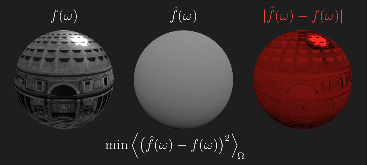
If we don’t need very high resolution, instead we may want to store a fast very low resolution approximation, we’ll call (\hat{f}). Note that (\hat{f}) is called “F hat” and the hat is common notation for approximations in statistics.
A 6-pixel (one for each face) cubemap or 8-value octahedral map works in many cases, but there are downsides which I won’t go into here.
So instead, let’s come up with a mathematical approximation (\hat{f}(\omega)) for our function (f(\omega)). A linear model like this is just about the simplest reasonable approximation that I can think of (aside from a flat constant):
Where we will precalculate and store our four coefficients: (c_0, c_x, c_y, c_z).
It might be obvious that you can think of the (c_0) term as an overall intensity, and the (c_x, c_y, c_z) as a directional intensity, for a particular direction. And if the length of the (\langle c_x, c_y, c_z \rangle) vector is larger than (c_0), you can get negative values (which will render in red below).
So how do we get these four coefficients? A quick idea might be to find the coefficients (c_0, c_x, c_y, c_z). that minimize the (sum/average/integrated) square error ((\hat{f}(\omega) - f(\omega))^2) against the original function or a high-resolution version. In other words, a good old fashioned linear regression. In this Python code we’ll sample some random directions and regress on those.
1 2 3 4 5 6 7 8 9 10 11 12 13
def encode_linear_coefficients(spherical_fn, num_dirs=8192, seed=None): dirs = generate_uniform_sphere_dirs(num_dirs, seed=seed) spherical_values = [spherical_fn(dir) for dir in dirs]
Calculate four linear coefficients for model with a constant
Construct the design matrix A: [1, x, y, z]
A = np.hstack((np.ones((num_dirs, 1)), dirs)) y = np.array(spherical_values)
Solve for least squares: A * c = y
coefficients, _, _, _ = np.linalg.lstsq(A, y, rcond=None)
return coefficients
These coefficients give us our fast, low-memory spherical approximation.
Well, we pretty much just reinvented spherical harmonic approximations! This is most likely something countless people have done without even realizing that what they did was equivalent to using SH.
Maybe it would be more accurate to say that this is a valid, though inefficient, implementation of a specific SH approximation. We would call this an (l = 1), or L1, spherical harmonics approximation, where “(l)” is the degree of the polynomial. You can also have an (l = 0) SH approximation, with a single constant like (\hat{f}(\omega) = c_0).
Higher (l) values will store coefficients for higher degrees of polynomials, for example (l = 2) includes coefficients for (x^2), (xy), (xz), (y^2), etc. Higher degree polynomials have a bit of extra complexity we’ll talk about later, but it’s still just a basic linear model, with a least squares fit!
Spherical harmonic approximations are actually nearly the blandest approximation model you could think of to represent a spherical function. If this is the first time you’re learning about SH, you might be thinking… why do we even use a special name for a basic linear model?
You may notice that I’ve been saying SH approximations rather than just SH. A big part of why we have a special name is the difference between the mathematical construct (spherical harmonics) and the application of them (SH approximations). Also part of the answer is due to the history of the application of SH to graphics, and due to the relationships with other things in math.
But there are two interesting properties of SH approximations that make them special compared to other linear models:
In graphics, performance is really important, so being able to do these things fast is a big part of why SH approximations are used at all.
As I’ll show shortly, the first property is because we are optimizing least squares over the uniformly weighted unit sphere, rather than any arbitrary distribution of x,y,z values.
The calculation of the coefficients is often called “encoding”. In a machine learning context this would often be called regression or fitting or learning or maybe compressing or mayyybe training.
When it comes to spherical harmonics, the fast method of encoding is specifically called projection.
Then evaluating the approximation function (\hat{f}) I’ll usually call reconstruction, but it could also be called decoding. In an ML context it might be called inference or estimation (or prediction, but that’s not really appropriate here, since we’re approximating something that’s known, rather than predicting something unknown).
We’re going to derive the fast encoding from scratch, for both the (c_0) term and the (c_x) term. The (c_y) and (c_z) terms are basically the same as (c_x). The derivation involves a small amount of calculus, but if you want, you can skip the L1 Encoding Derivation section, and go to L1 Encoding Rules (Projection).
Typically to minimize a function with multiple parameters, you’d need to jointly minimize every parameter. But let’s see what happens if we start by optimizing just (c_0) on its own.
We want to find the (c_0) that minimizes least squares errors. This is written as:
In this case, the integral over big-omega (\Omega) means we’re integrating over the sphere, and the little omega (\omega) represents a direction.
But rather than using spherical integrals, we’re going to switch to spherical averages (means), because minimizing the integral of squared error is the same as minimizing the average squared error. The notation I will use for a spherical average uses the angle brackets (\langle , \rangle_\Omega). The more standard notation drops the (\Omega) subscript, but I think it’s clearer to keep it, especially to distinguish between vectors which also use the angle brackets.
Formally, the average is the same as the integral divided by the surface area of the sphere:
Doing this means that we can ignore the surface area of the sphere, which makes the math and programming easier.
I am not the first person to use spherical averages to simplify SH, and I think Graham Hazel did the best job fleshing this out, but I’ll link to that article in the Bridging the Gap section. Anyway, so we are trying to solve:
To find a minimum, we need to find the value of (c_0) such that the first derivative of this is zero.
Typically to minimize you’d also worry about local minima or finding maxima, but as we’ll see, there is only one solution here - the function is convex.
The derivative of an average is the average of the derivative:
Now let’s focus on (\frac{\partial(\hat{f}(\omega) - f(\omega))}{\partial c_0}).
(\frac{\partial f(\omega)}{\partial c_0}) is zero, because (c_0) is unrelated to the original function.
Expanding (\hat{f}(\omega)), we have (\frac{\partial(c_0 + c_x \omega_x + c_y \omega_y + c_z \omega_z)}{\partial c_0}), which is simply (1).
Divide by 2, plug in the definition of (\hat{f}(\omega)) again, and separate all the average terms, and we have this:
Now the average (\langle c_0 \rangle_\Omega) is of course (c_0), it’s a constant. (\langle c_x \omega_x \rangle_\Omega) is 0, because it’s symmetrically distributed over a sphere (for every (\omega_x) value, there is also a (-\omega_x) value), and same for the other two terms. So we get this wonderfully intuitive and easy to calculate value.
The constant is just the average value of our function over the whole sphere!
Not only that, as we alluded to earlier, the optimal (c_0) value is not dependent on any of the other coefficients - they can be optimized independently.
Like the previous derivation, we would first take the derivative and set it to zero. And then starting with the chain rule and power rule and move the average outside the derivative:
Focusing on the inner derivative term, again we separate the terms, such that
(\frac{\partial f(\omega)}{\partial c_x}) is still zero, because (c_x) is unrelated to the original function.
(\frac{\partial\hat{f}(\omega)}{\partial c_x} = \frac{\partial(c_0 + c_x \omega_x + c_y \omega_y + c_z \omega_z)}{\partial c_x}) and that is simply (\omega_x), because it’s the only term with (c_x).
Expanding (\hat{f}(\omega)) and separating the average terms:
Because of spherical symmetry, every average term is zero except the (\omega_x^2) one, because (\omega_x^2) is non-negative everywhere, which simplifies to:
Because (\omega) is a unit vector, we know that the length and length squared are one:
So we can also say that the average squared values add up to 1:
Since a sphere is symmetrical for all the three axes, the averages are all the same: (\langle \omega_x^2 \rangle_\Omega = \langle \omega_y^2 \rangle_\Omega = \langle \omega_z^2 \rangle_\Omega), and we can substitute that in, so (3 \langle \omega_x^2 \rangle_\Omega = 1). That gives us:
Now you start to get a sense for why this is called “projection”. It looks like projecting the function onto the (\omega_x) v
正文由 探How 从来源站点 RSS 同步,内容未经改写;遇到排版缺失或需要图片、视频时请以原文为准。