The election is almost a week away, and the people demand to know what will happen. This, as always, leads to a lot of polls and a lot of frantic speculation. One problem with this, though, is that a lot of people out there are passive consumers of news. They read what happens to cross their feed, and so what they see will be a function of what goes viral. The problem with this is that the most viral polls are not the most representative polls. I explored this in the old Twitter days, but I thought it was worth revisiting now.

Given that Musk has absolutely destroyed the Twitter API for academic use, I had to instead rely on what happens on Bluesky. Bluesky is well known for having a clear left-wing tilt, while also being the posting retirement home for elder millennials. So this is not exactly a representative sample of what goes viral in polling, but it is in line with what I found a long time ago looking at Twitter. In brief, I scraped the last 90 days of posts from @usapolling.bsky.social, who appears to be the most active “polling distribution” account on Bluesky. After that, I used an LLM and an overly complicated prompt (see below) to extract the information in each post. I then calculated the margin for the race(s) in each post and finally calculated the average margin for each race (Dem-Rep). To further simplify things, this analysis focuses only on posts that included a single general election poll. Nothing is perfect, but I probably should be spending time working on publishable research and lectures anyway.

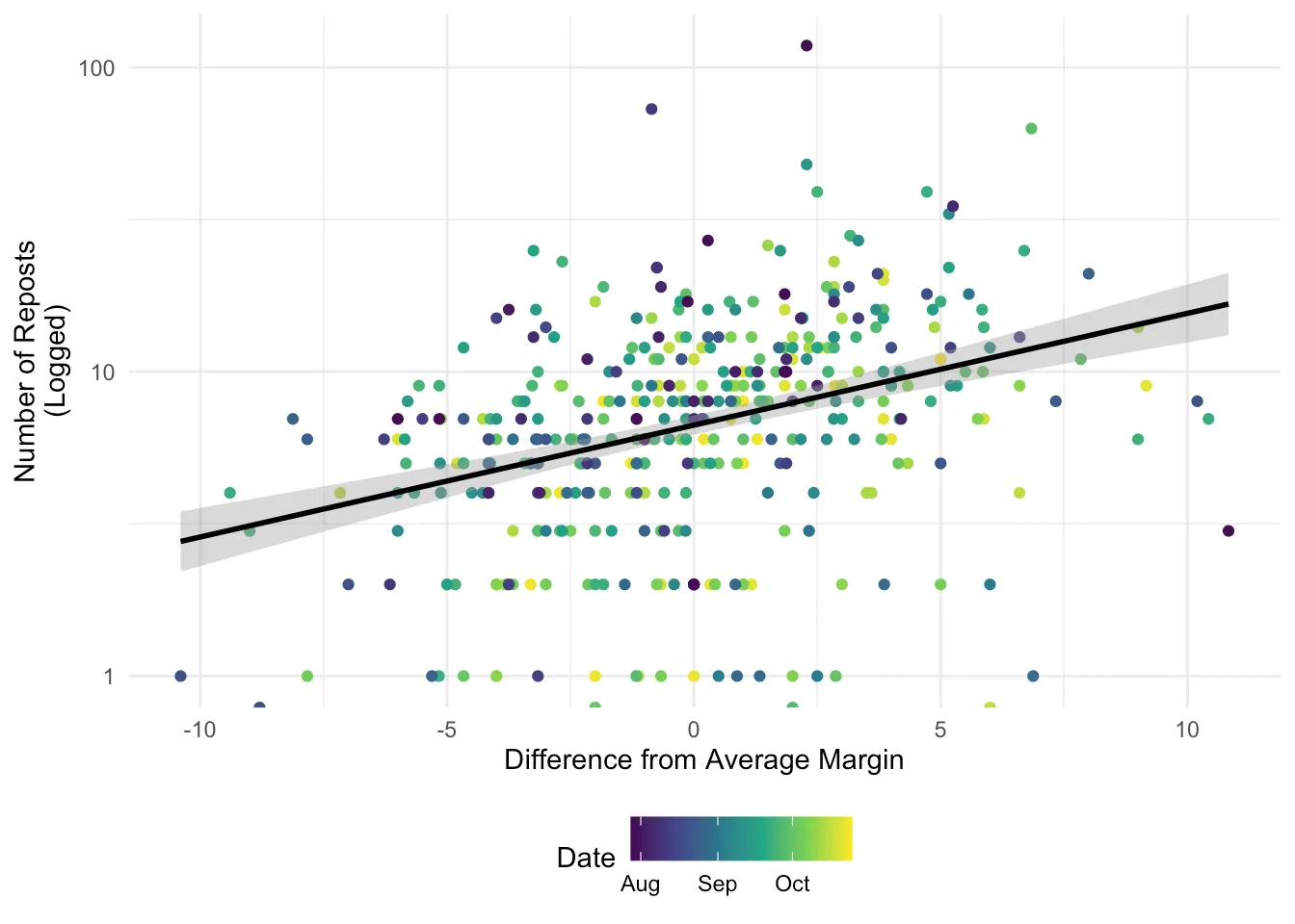
Figure 1 shows the number of reposts for each poll post by the difference from the average margin for that race. Moving to the right along the x-axis means that a poll was more favorable for Democrats than other polls in the race. I’ve filtered this to include only races where there were multiple polls posted. The black line shows a line of best fit, indicating that as polls become “better” for Democrats (further from the average poll in that race), they tend to be reposted more.

library(tidyverse) library(lme4) library(broom.mixed) library(huxtable) library(ggeffects)

df <- read_csv(here::here("blog/data/election_polling.csv"))

df <- df |> mutate(Date = as.Date(time)) |> mutate( ID = as.factor(ID), Seat = as.factor(Seat), Date_Numeric = as.numeric(Date) - min(as.numeric(Date)) ) |> mutate( ID = case_when( ID == "Generic" & Seat == "GenericCongress" ~ "Generic-Congress", .default = paste0(ID, "-", Seat) ) ) |> filter(!(ID == "TX" & Seat == "GenericCongress"))

df |> filter(N > 1) |> ggplot(aes(x = Margin_Diff, y = reposts, color = Date)) + geom_point() + scale_y_log10() + geom_smooth(method = "lm", color = "black") + theme_minimal() + theme(legend.position = "bottom") + scale_color_viridis_c(trans = "date") + labs( x = "Difference from Average Margin", y = "Number of Reposts\n(Logged)" )

Figure 1: Reposts by Difference from Average Margin

It is also possible to look at race-level variation. In Figure 2, I show the same style of plot broken out by race (and one for just generic congressional polls). I’ve only included races where there were at least 10 polls (or else it is just overwhelming). We see the same pattern for almost every one of those races: the most viral posts are the ones that favor Democrats more than the average post (with the one exception being the NC Senate race for some reason).

df |> group_by( ID ) |> filter(N > 10) |> ggplot(aes(x = Margin_Diff, y = reposts, color = Date)) + geom_point() + scale_y_log10() + geom_smooth(method = "lm", color = "black") + facet_wrap(~ID) + scale_color_viridis_c(trans = "date") + labs( x = "Difference from Average Margin", y = "Number of Reposts\n(Logged)" ) + theme_minimal() + theme(legend.position = "bottom")

Figure 2: Race by Race - Reposts by Difference from Average Margin

We can go a step further and estimate a model predicting the number of reposts based on the Dem-Rep margin, the post margin minus the average margin, and the date the post was shared. To account for the fact that we are mixing a bunch of races together, I estimate a model with random intercepts for each race (I exclude the generic congressional race and include only races with more than 5 posts). The predicted number of reposts across values of the difference from the average margin and the margin itself is displayed in Figure 3. Again, this shows that the distance from the average margin is what dictates post virality, with the margin itself being relatively unrelated.

mod <- lmer( log(reposts) ~ Margin_Diff + Margin + Date_Numeric + (1 | ID), data = df, subset = reposts > 0 & N > 5 & N < 50 )

ggpredict(mod, terms = c("Margin_Diff [-10:10] ")) |> plot(show_title = FALSE) + scale_y_continuous(limits = c(0, 20)) + labs( x = "Difference from Average Margin", y = "Number of Reposts" ) ggpredict(mod, terms = c("Margin[-20:20]")) |> plot(show_title = FALSE) + scale_y_continuous(limits = c(0, 20)) + labs( x = "Dem-Rep Margin", y = "Number of Reposts" )

#huxreg(mod)

(a) Predicted Reposts Based on Diff from Avg Margin

(b) Predicted Reposts based on Margin

Figure 3: Predictions from Random Intercept Model

If we include random slopes as well, this can tell us something interesting about which races are most likely to go viral right now. In Figure 4, I show the random effects of a model with random slopes and random intercepts. This can be read as indicating how different each race is from other races. For example, the TX-Senate race is likely to get more reshares in general, and a post that shows the Democrat up is going to go especially well. In contrast, no one cares about the Pennsylvania governor’s race (which might have to do with Bluesky’s feelings towards Josh Shapiro).

mod <- lmer( log(reposts) ~ Margin_Diff + Margin + Date_Numeric + (1 + Margin_Diff | ID), data = df, subset = reposts > 0 & N > 5 & N < 50 )

sjPlot::get_model_data(mod, type = "re", sort.est = "Margin_Diff") |> mutate(facet = ifelse(facet == "ID (Intercept)", "Intercept", "Slope")) |> ggplot(aes( x = estimate, xmin = conf.low, xmax = conf.high, y = reorder(term, reihe) )) + geom_pointrange() + facet_wrap(~facet, scales = "free_x") + theme_minimal() + labs(y = "Estimate", x = "")

Figure 4: Random Effects Estimates

NoteAI Use

The Python code (below) was written using OpenRouter’s Auto Router, which routes LLM requests to models. It routes requests to different models based on a classification model run by OpenRouter, aiming to minimize cost while maximizing quality. I have it set to use only Zero Data Retention models (for what that is worth) and to the “High” cost tier. The R code and prose were written by hand, with one run of an LLM to identify typos and grammar issues in the prose.

If you are curious, below is the entire Python code used to scrape the posts and extract the data. It is very overly complicated and is broken up into chunks that made sense in my brain.

This simply uses the atproto library to grab the last 90 days of posts. I did a bit of quick filtering, removing blank posts (probably images) along with posts that do not have a number in them.

import datetime as dt import pandas as pd from atproto import Client from dotenv import dotenv_values

config = dotenv_values(".env") client = Client() client.login( config["BLUESKY_HANDLE"], config["BLUESKY_PASSWORD"], )

cursor = None end_date = dt.datetime.now(dt.timezone.utc) - dt.timedelta(days=90) posts = []

Fetch the author feed until the date cutoff or the final page.

while True: timeline = client.get_author_feed(actor="usapolling.bsky.social", cursor=cursor) if not timeline.feed: break

for feed_view in timeline.feed: created_at = dt.datetime.fromisoformat(feed_view.post.record.created_at) if created_at <= end_date: break

posts.append( { "text": feed_view.post.record.text, "time": created_at.isoformat(), "reposts": feed_view.post.repost_count, } ) else: cursor = timeline.cursor if not cursor: break continue break

polling_data = pd.DataFrame(posts)

This sets up the schema that is used to extract information from the post, along with the prompt. The Pydantic part of this is used to validate the response, make it easier to process, and help guide the model. This is the most vibe-coded part.

import re from decimal import Decimal from enum import Enum from typing import Annotated

from pydantic import BaseModel, ConfigDict, Field, ValidationInfo, model_validator

class Party(Enum): Dem = "Democrat" Rep = "Republican" Indep = "Independent" Other = "Other"

class Stage(Enum): General = "General" Primary = "Primary"

class Seat(Enum): House = "U.S. House of Representatives" GenericCongress = "Generic congressional ballot" Senate = "U.S. Senate" StateHouse = "State House / Assembly / House of Delegates" StateSenate = "State Senate" Gov = "Governor" Other = "Other"

class PostType(Enum): Candidate = "Candidate vote intention" Generic = "Generic party ballot" Approval = "Approval or favorability" Issue = "Issue or ideological preference" Forecast = "Forecast or polling average only" Other = "Other" Unclear = "Unclear"

class ExclusionReason(Enum): NotVoteIntention = "Not an election vote-intention poll" ForecastOnly = "Forecast or average only" MarginOnly = "Margin only" MissingPercentages = "Fewer than two explicit candidate or party percentages" MultipleScenarios = "Alternative scenarios for the same race" Unclear = "Insufficient evidence to classify or extract"

class Universe(Enum): Registered = "Registered voters" Likely = "Likely voters" Adults = "Adults" Other = "Other explicitly described population"

EvidenceExcerpt = Annotated[str, Field(min_length=1)] Evidence = Annotated[list[EvidenceExcerpt], Field(min_length=1)]

class EvidenceModel(BaseModel): model_config = ConfigDict(extra="forbid")

@model_validator(mode="after") def require_field_evidence(self): for field_name in type(self).model_fields: evidence_name = f"{field_name}_evidence" if evidence_name in type(self).model_fields: value = getattr(self, field_name) evidence = getattr(self, evidence_name) if value is not None and ( not evidence or any(not excerpt.strip() for excerpt in evidence) ): raise ValueError(f"{field_name} requires supporting evidence") if value is None and evidence is not None: raise ValueError(f"Unknown {field_name} must have null evidence") return self

class Candidate(EvidenceModel): name: str = Field( min_length=1, description="Candidate surname/name or generic party label exactly as written; never expand names.", ) party: Party | None = Field( description="Null if unsupported; Other and Independent are not unknown." ) party_evidence: Evidence | None = Field( description="Verbatim party label or candidate line with a party marker; null if unknown." ) percentage: float = Field( ge=0, le=100, description="Poll support percentage, not a margin, forecast, or model result.", ) percentage_text: str = Field( description="Exact percentage token, including % or percent, e.g. '46.5%'." ) candidate_evidence: Evidence = Field( description="List of verbatim excerpts linking this name/party label to its percentage; at least one excerpt must contain both together.", )

@model_validator(mode="after") def check_candidate_evidence(self): if not any( self.name in excerpt and self.percentage_text in excerpt for excerpt in self.candidate_evidence ): raise ValueError( "At least one candidate_evidence excerpt must contain both the name and percentage text" ) match = re.fullmatch( r"(\d+(?:.\d+)?)\s*(?:%|percent)", self.percentage_text, re.IGNORECASE ) if match is None or Decimal(match[1]) != Decimal(str(self.percentage)): raise ValueError("Percentage must match the quoted percentage token") return self

class Race(EvidenceModel): race_evidence: Evidence = Field( description="List of verbatim excerpts establishing this matchup; a shared state/office he