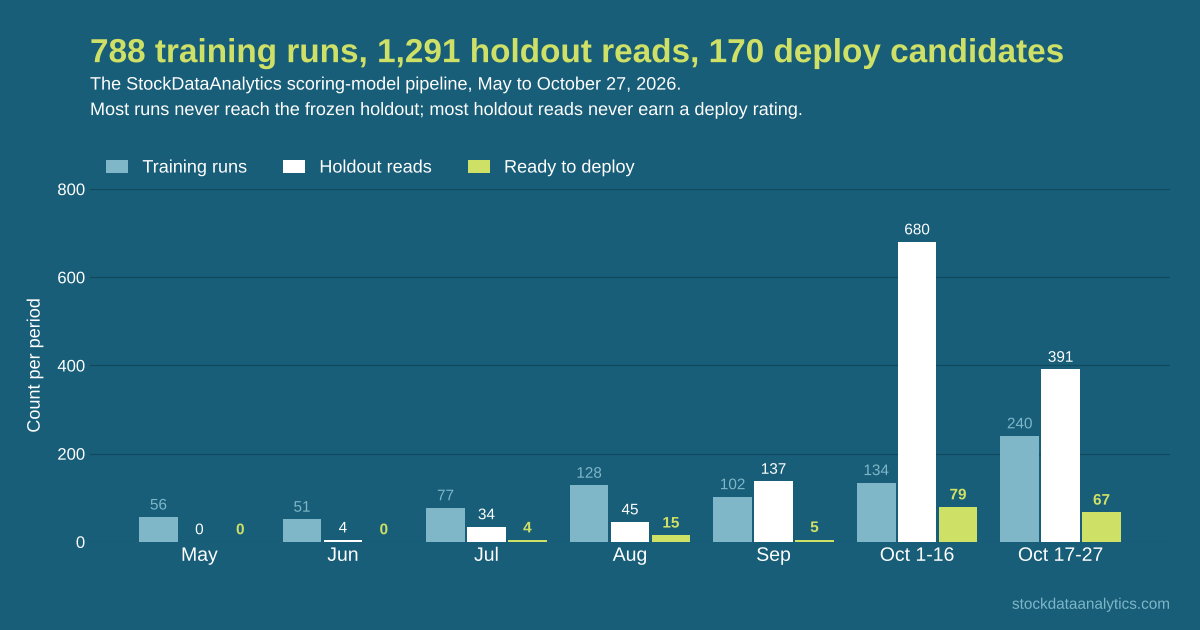
Training a stock scoring model 800 times taught me six ways it fools itself

27 min read

How We Train Stock Pattern Scores: 600 Runs, 6 Overfitting Traps

Every chart pattern score on StockDataAnalytics.com comes from a training pipeline that has run nearly 800 times since May 2026. It screens a few hundred candidate features per pattern, fits an additive model, tests it on a frozen holdout it never trains on, and marks a model ready for a live parallel run only if it beats the one already live on that holdout. One pass over all sixteen pattern detectors takes about three quarters of an hour on a single Mac (35 minutes when the samples were half the size). Ten of our twenty production detectors ran models that came out of it by mid-October.

Here is what surprised me when I stepped back and looked at what I had built. Most of the code is not modelling. The training tree is about 88,000 lines of Python, and the part that fits a model is a small slice of it. The rest is the ruler: the splits, gates and ledgers that decide whether a model is real. That is because the edge we are looking for is small. A typical fitted model's out-of-sample rank correlation with the two-week outcome is about 0.03; a good one reaches 0.08 or 0.09. At those sizes, telling a signal from a lucky draw of the data is the whole problem.

One caution belongs up front. The holdout numbers in this article are strong; the live numbers so far are not. On this year's production rows, measured within day and market at a one-week horizon, the pattern quality score has ordered market exposure rather than outcome, and only one detector in sixteen orders excess return the right way with an interval that excludes zero. The last section says what that means for the deploy rule.

It has to produce a score where a 36 wins more often than a 24. If it does not, the ranking is noise and so is the email.

The target I set in spring was a top band that wins more than 75% of the time. In October I downgraded that from a gate to an aspiration, because absolute goals had started to block incremental progress. The gate now is a simpler question. Is this candidate better than what is live, on the worse of two out-of-sample windows, by enough to matter?

One run takes each enabled detector (16 of 18 today) through the same chain, and a single detector's pass takes eight to ten minutes.

"Nightly" is a misnomer by now; a training batch is 20 to 40 iterations and runs through the day. On October 14 the history shows thirty runs.

Each detector's pass (a "leg") gets one strategy, which fixes the target (the measure of trade success the model is fitted to), the scoring mode and the market regimes it fits on; everything else is held constant, so two runs of the same strategy differ only by their random seeds. There are six targets to choose from, because the first one we used was wrong. A June post-mortem found that raw two-week return in a rising market is mostly beta (how much of the index's move a stock takes on): a model fitted to it could look predictive simply by liking volatile stocks. So the pipeline keeps six targets in play, among them return minus the index and a triple-barrier label (did the trade hit +1.5 ATR before −1.0 ATR within ten trading days).

The chain itself: pull a sample of detections and their outcomes; screen the candidate features; fit the model and translate it into a points ladder; ask whether the fit beats the best of many lucky tries; decide whether a read of the frozen holdout can resolve anything; read it; rate the result against the live model.

Here is a real leg from the run that produced one of the models installed on October 15: inverse head and shoulders, fitted to the triple-barrier label. Extract, 4 minutes. Feature screen, 2 minutes, 206 candidates left. Fit, 79 seconds, clearing the selection bar with an out-of-fold correlation of 0.0629. Holdout read allowed (seventeen earlier reads on that holdout, all logged). Live rule: the current model wins 54.5% at 36+; the candidate wins 71.6%. Deploy. Eight and a half minutes, start to finish. That is the unit of work, it is cheap, and taking many cheap shots is why most of the machinery below exists.

The split is one chronological cut: the oldest 50% of rows train the model, the next 25% validate it, the newest 25% is a holdout the model never sees until the final read, and the last 14 calendar days before each boundary are discarded so a two-week outcome cannot leak across.

Every training row is one detection (one stock, one day, one pattern) joined to the simulated trade that followed it. Almost every detector samples 90,000 rows from January 2022 to March 19, 2026. For the October 15 models, the cut worked out to training from early 2023 to August 2024, validation to mid-2025, and holdout from mid-2025 to March 2026.

The holdout is frozen: its rows are recorded by pattern, ticker and date, and every later extract rebuilds exactly those rows. The first version recorded database ids instead. A backtest deletes and reinserts the detections table with new ids, so a frozen holdout could silently shrink, and on September 22 it did: one detector's freeze matched 0 of 33,013 rows and nothing in the run said so. Now a freeze that resolves fewer than half its keys refuses to start the run.

Past the holdout sits a fourth slice, the forward period, which begins April 9, 2026. Training and the holdout read never load it; it is read once per promoted model, and by the parallel run.

Each candidate feature goes through fourteen checks, and the one that changed what the pipeline finds is a test of whether the feature predicts which stock to buy or merely when to buy.

Most of the battery is what you would expect: correlation with the outcome on training and validation, effect size between winners and losers, the same sign within bull and bear regimes and across chronological blocks, and a correlation with 20-day volatility no higher than 0.40, so the feature measures the pattern rather than the volatility class. One exclusion is deliberately loud. Any column whose name says it was measured over the outcome window raises an error and stops the run; four such columns were found in September. A feature that knows the future should stop the pipeline, not lose a tier.

The biggest change came in October, from a suspicion I had carried for months. Too many models leaned on market-wide features: index correlation, sector co-movement, the volatility regime. They predicted well in validation. I suspected the models were learning the calendar.

On October 5 we measured it on the seventeen models that had reached a holdout read. Each model's score spread was split into the part explained by which day a detection happened on and the part explained by ranking stocks against each other on the same day. The median validation win-rate spread between top and bottom score bands was 13.5 points; the within-date spread was 4.4; on the holdout both collapsed to about 2 points. Half of the validation spread was market timing, and the timing did not transfer.

Underneath that is an independence problem. The p-values had treated roughly 10,000 rows as independent observations. For a market-wide feature, every detection on one day moves together, so the real number of observations is closer to the number of trading days: around 400. Every significance test was overstated for exactly the features that transfer worst.

Three changes went in against it. A date-share gate rejects any feature with more than 30% of its variance between days. Significance is tested over days rather than rows: the correlation is computed within each trading day, and the mean of those per-day correlations is what gets tested. And the direction and consistency checks are recomputed on the same per-day statistics. The roster-wide admitted pool went from 1,407 features to 1,006, 28.5% fewer, each measured on the question that matters. With about 420 trading days in the window, the smallest within-day effect the screen can distinguish from zero is about 0.02, and only more days (not more rows per day) shrink that floor.

Multiple testing is controlled with the Benjamini-Hochberg procedure (which caps the share of false discoveries rather than the chance of any single one) at 10%. It replaced Bonferroni in June, because Bonferroni across a few hundred features had demanded p-values no real effect in this data reaches.

The model is a gradient-boosted tree ensemble constrained so hard that it stops being a forest: no tree may split on more than one feature, so the whole model is a sum of one-dimensional curves, and each curve can be read off as an exact table of thresholds and points.

For its first month the fitter tried the obvious workaround: fit an unconstrained "teacher" model and translate it into a ladder afterwards. The translation lost most of what the teacher learned. On May 29 the teacher went, and the fitter started fitting the ladder's shape directly.

Which features get in is decided twice. The screen's tiers are the first gate. The second is inside the fit, and it is where most features die: the fit is repeated nine times with different seeds, each time on the real features plus a shuffled "shadow" copy of every candidate, and a real feature is admitted only when its importance beats the 85th percentile of the shadow columns in at least five of the nine fits.

Cross-validation uses five contiguous date blocks, with training rows within 16 calendar days of a test block purged and the 10 days after it embargoed, and hyperparameters are re-tuned inside each fold.

Each component holds at most 12 structure, 10 volume and 10 breakout features, and the raw sums are scaled to the customer range by dividing by the 97th percentile of the training distribution. That percentile was 99.5 until October 4, and audits found that 419 of 421 fits never used the full score range: to reach 36, a detection had to sit near the 99.5th percentile on all three components at once, which almost nothing does. Lowering it changes no ranking; it only moves rows into the bands the deploy rule can judge. Finally the fitter generates the detector's scoring code, runs it in isolation against every row it was fitted and validated on, and requires a 100% match. The code that ships is the code that was tested.

Three tests must all pass: the fit's p-value survives correction against every earlier attempt on the same detector, its correlation beats the expected best of N random tries, and its top band beats the rest of the validation rows by more than a round-trip trade costs.

By October a busy detector had dozens of fits on the same data, and the best of fifty fits on noise will always look like something. The second test uses the Bailey and López de Prado approximation for the expected maximum of N draws, and N is not the raw count: earlier attempts are clustered by how similar their predictions are, so twenty near-identical fits count as fewer than twenty. The third test asks whether the top 5% to 10% of validation rows beat the rest by more than a 0.3% round-trip cost.

Two bugs in this bar show what "wrong" looks like here. Until July 3 the second test used the absolute value of the correlation, and a three white soldiers model with a correlation of −0.0634, ranking stocks backwards, passed with a z-score of +9.83. And until August 27 the third test asked only whether the top band's mean return was above zero; a bull flag model passed with a 410-row top band averaging 0.96% against a baseline of 1.12%. A band holding most of the population passes trivially, because its mean is the baseline. A gate audit in July counted 33 tests that could veto a model. Today exactly four can.

A read is withheld when fewer than 50 holdout rows are projected to land in the top band, when the candidate's feature set overlaps 80% or more with the last model read on that holdout for the same target (unless its projected top band has grown by a quarter), or when the candidate's own validation numb