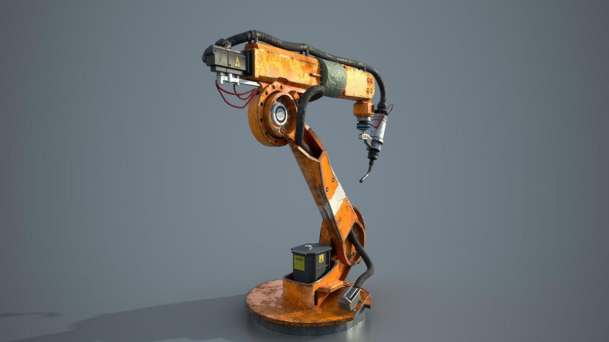
End effector action policy outputs to robot actuation

Avi

Oct 26, 2026

1

Share

Introduction

While building out-of-box support for fine-tuning and testing of open-source VLAs like π0 for Lagrangian, one of the key challenges I came across was my lack of appreciation for the complexity involved in transforming the model output to actuator controls signals for the robot.

My naive understanding, some stemming from the lack of details in the original π0 paper but mostly perhaps because of my own lack of understanding, was that the model output was simply a delta in generalized position coordinates of the 7/8-DOF arm + gripper.

However, after facing interfacing challenges between the pre-trained π0 checkpoint output and controlling the 7-DoF arm I wanted to, along with observing some weird behavior, I realized I couldn’t be further from the truth.

The supported Lagrangian pre-loaded π0 checkpoint uses HuggingFace’s LeRobot π0 Libero base model. A help doc in the LeRobot Github repo clearly describes the output control as follows:

Actions: Continuous control in Box(-1, 1, shape=(7,)) — 6D end-effector delta + 1D gripper

The proprioceptive input on the other hand is described as follows:

observation.state — 8-dim proprioceptive features (eef position, axis-angle orientation, gripper qpos)

The control output can be interpreted as delta of the Cartesian position and orientation (in Tait-Bryan representation) of the end effector (aka eef) pose in world frame.

A regular Franka Emika Panda arm model has total 8 actuators (7 for the arm + 1 for the gripper), 7 arm joints & 2 gripper joints (with 1 of the gripper joints being redundant given the equality constraint imposed between the 2 gripper joints).

Each of these above 8 actuators are SISO (single control input and single control output) joint-based actuators, which naturally drive the above joints.

Now given π0 policy’s end effector control output, a natural question arises regarding how the 6-dim target end effector delta state is to be transformed to the 7-dim control input required to actually control the robot arm.

The remainder of this post will sketch out this procedure in as much exacting detail as possible, deriving everything from first principles.

Say from some control policy (like π0) we have the deltas in end effector state (ignoring the gripper dynamics for now given they’re simply generalized position deltas), in terms of Cartesian position and Euler (Tait-Bryan) orientation angles. The policy is essentially saying, move whole arm such that the commanded end effector motion is complied with, that I don’t care about the specifics of the whole arm but mainly the end effector which is mainly what effects my task.

To be able to derive the actuator control input (which is our goal) we must first derive the joint space generalized forces τ which cause the same motion as that commanded by the policy.

To obtain τ we first determine the end effector’s target acceleration (in the world frame) to comply with the commanded motion.

We use PD control here for this, using the commanded/target position as input. The general equation for PD control derivation of target acceleration is as follows:

Here the command acceleration vector (a_c) is a 6-dimensional spatial motion vector, the top 3 components representing the eef frame acceleration and the bottom 3 components representing the eef frame angular acceleration.

Focusing on position only first, assume a target Cartesian position x_d and Cartesian target velocity v_d, both expressed in the world frame, then e_p, e_v are:

For calculating the error components for the orientation the equations are a bit more involved. This is because the rotation orientation of the eef frame cannot be directly derived as a delta between the rotational states whatever numbers & representation be used to capture it.

Assume that the world frame is represented by W, the current eef frame is represented by E and the desired eef frame orientation is represented by D.

Here R^{-1}=R^T given the orthogonality of rotation matrices. Now, from the above the rotational adjustment needed is:

Here the term R_e can be taken to be the error correction rotation transform which transforms between the current end effector frame orientation and the desired orientation.

To be able to represent this in the 3 component vector representation we derive the axis-angle representation of this rotational error term R_e via the logarithm method.

Now, onto the angular velocity error term e_v[3:6]. To obtain this we can simply use the difference between the angular velocity vectors. Hence:

Putting it all together to obtain the e_p & e_v terms for the above PD control equation:

For π0-like control policies, desired acceleration and desired velocity terms will be set to zero in most cases.

Note, this does not mean that the K_d term will be irrelevant as the end effector’s current velocity still effects the commanded acceleration inversely due to the negative sign.

Now from the above section we have a_c, the command acceleration for the end effector required to comply with the command.

Given that the policy output commands and the term a_c describes the end effector motion only (in the world frame), to derive joint space generalized forces τ, we need some way to transform between the end effector motion and force terms represented in the world frame. Operational space control (OSC) provides a way to do this.

The idea behind OSC is to provide a framework where the robot can be controlled directly in the task aka operational space (in our case, the end effector motion in world frame) which can then be converted to robot joint level motion and forces to be used for actually commanding the actuators. Exactly what we need.

We derive OSC equations here from first principles. Let’s assume a vector function ϕ which transforms between generalized joint position vector q to the end effector Cartesian position and orientation x i.e.:

We can differentiate on both sides to obtain:

In our case, we assume that n_x < n_q given that the end effector Cartesian pose vectors requires 6 numbers in total to represent while the robot arm is assumed to have anywhere from 7-8 degrees-of-freedom.

This forms the basis of our transform between the 2 sets of objects we have, joint space motion and force vectors and end effector’s / task [world] frame motion and force vectors.

We now have a way to obtain the generalized joint space forces using the end effector acceleration a = a_c.

We can stop here for our purposes, assuming that the generalized inertia matrix H and the generalized bias force C is known. However standard formulations of OSC dynamics equations like to frame the equations using the task space inertia matrix and the task space force. To obtain this we keep going.

From the principle of virtual work, the virtual work performed by the task space end effector force to perform the command motion should be equal to that performed by the generalized forces on the joint motion. In equations this is:

Here given the prior assumption of J having full-row rank the J^T is assumed to have full-column rank & have the pseudo-inverse as well.

This is the final formulation used to describe operational space control dynamics. We can inject PD control command acceleration we derived in the prior section to obtain:

Now, we’re all set. The PD control command acceleration from (1) can also be injected into (20) to obtain the generalized joint space forces:

All that remains is deriving the actuator control inputs. To obtain these, we work with Mujoco’s actuator model with some restrictions for the robot arm problem domain:

All actuators for the robot are assumed to be SISO (single-control-input-single-control-force-output) (this used to be generally true in Mujoco until very recently actually).

All actuators are assumed to have joint transmissions.

All joints associated with the actuators are assumed to be hinge joints.

Now given the above assumptions, the transmission length for each actuator is given simple by:

Using the principle of virtual work again, the virtual work done by the actuator force output on the transmission should be equal to that by the generalized forces on the joint space configuration. Hence:

The transmission length Jacobian can be further simplified using (26), after which we have:

Referencing the Mujoco documentation for actuator modeling again, we have:

Here we want to derive u which is our actuator input control vector. Using (26) to further simplify (29), we have:

Finally, we have the actuator control input for the robot arm after starting off from the end effector position delta commands for Cartesian position and orientation in the world frame.

There’s an additional matter. The Jacobian transforming between the end effector motion and joint space motion is a rectangular matrix of shape [n_x,n_q] . While we assumed n_x < n_q and full-row rank for this matrix, given its shape we have a nullspace of dimension n_q - n_x.

This means that we can perform hide some additional joint space motion in this null-space which would still result in remaining compliant with the commanded motion for the end-effector / task space.

This statement can be formally captured in math by modifying equation (19) from above:

We can use the equation (23) to better understand and even formally define τ_null. We want this null-space force to produce no motion (or acceleration) for the end effector. This can be derived by replacing (33) in (23):

Here for the null-space force to generate no motion in the end-effector we need:

Equation (39) must always hold for τ_null.

Given this, the null-space generalized force can be seen as not interfering with the task objective motion commanded by the policy.

Now, I think this is quite neat and is used for many applications, listing a few here:

Joint configuration compliance including joint limit avoidance

Of course, having this null-space available doesn’t guarantee any of the above additional requirements as depending on the configuration this null-space may not be as large, but it’s a nice little extra playground to be able to use.

Further, we derive a projector matrix N_null which can project between any generalized joint space force vector τ_null and project it the null space for compliance, hence:

One possible null-space projector can be:

You can start RL fine-tuning and testing open-source VLAs like π0, π0.5, π-fast, Gr00t with Lagrangian now, with the ability to setup multi-GPU workloads, configure custom reward functions, maintain-mix-match checkpoints and datasets, track workload logs and progress metrics over the Lagrangian dashboard & more.

The fine-tuning and testing workload setup configuration & capabilities can be further checked via the API docs.

If interested in obtaining an API key for trial, contact us via Lagrangian homepage contact form or even feel free to email me directly at: avideepgabhawala@gmail.com.