Scaling Hierarchical Networks

Since Richard Sutton’s influential essay in 2019, the concept of the bitter lesson has guided much of modern progress in AI. This concept espouses general methods that leverage computation and learn with scale, as free of human-engineered priors as possible. Our interpretation is that, fundamentally, intelligence is about learning from raw data: autonomously finding patterns, building abstractions, and developing meaning from messy low-level inputs, ideally end-to-end and as data-efficiently as possible. As AI advances into complex domains such as science, robotics, and biology – where data is scarce and often difficult for humans to understand, let alone engineer for – internalizing this philosophy to develop more general learning algorithms is more important than ever.

Language models are perhaps AI’s biggest success story today, and largely embrace the bitter lesson. Their abilities are largely attributable to scaling a few simple algorithms such as the Transformer architecture, next-token prediction, reinforcement learning, and test-time computation. However, they still rely on hand-crafted encoding steps such as tokenizers, which severely hinder their ability to learn end-to-end from the underlying data. Towards unlocking another step change of scaling, we believe that developing byte-level language models is foundational for AI progress – not just for improving standalone LLMs, but also as a litmus test for general learning methods. If we can’t even learn language well from characters and bytes, what right do we have to make progress on the next frontier?

In 2025, we developed the concept of hierarchical networks (H-Nets), which not only addressed tokenization in language models, but took a step toward even more general-purpose architectures that could learn from raw data across different modalities. We’ve since significantly improved the technology of H-Nets and are excited to share their capabilities! In this series of two posts, we’ll dig into new results and discuss the implications.

In this first post of a two-part series, we’ll explore scaling laws for H-Nets and their qualitative behaviors.

In the next post, we’ll do a deeper exploration of a larger range of models to understand better why H-Nets can be so much more efficient for language modeling.

Altogether, our results provide evidence that H-Nets are a foundational architecture that truly aligns with the bitter lesson, learning meaning directly from raw data and significantly improving efficiency and scalability. This research agenda represents a major opportunity to advance how AI can learn from all data, and we couldn’t be more excited to push the frontier!

We introduced hierarchical networks (paper, blog) last year as a new end-to-end architecture that models multiple levels of abstraction in data, showing promise in language modeling and beyond. In a nutshell:

Hierarchical networks (H-Nets) compress data through a recursive, data-dependent dynamic chunking process.

The terminology was inspired by the existing concept of chunking in cognitive psychology, which is an essential part of human intelligence. We believe it is also necessary for the frontier of artificial intelligence.

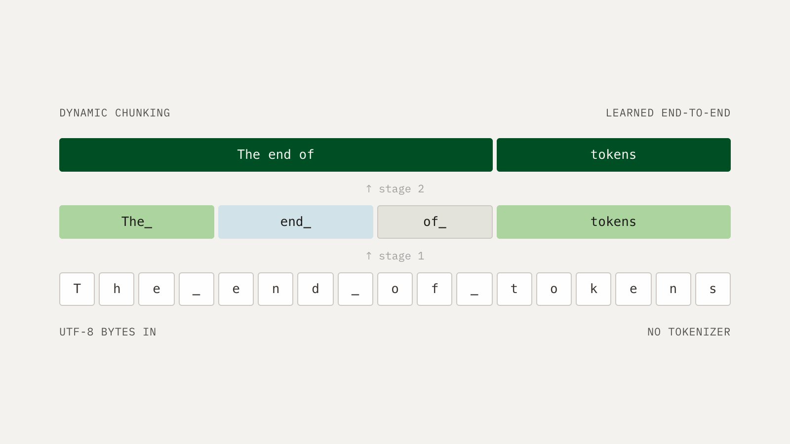
In the context of language modeling, the idea is to build new learning primitives that allow models to recursively chunk low-level data into higher-level meaning: characters into words, words into phrases, phrases into concepts.

In the context of this post, for the most part, one can think of hierarchical networks as replacing tokenization. Instead of pre-processing data from bytes into tokens (fixed chunks of bytes), H-Nets perform the chunking dynamically directly inside the model. Furthermore, the signature characterization of H-Nets is that they hierarchically perform this chunking end-to-end. In contrast, standard tokenized language models and even other alternatives (some of which we’ll see in Post II) employ multiple stages of training, and the process of chunking / tokenizing the data is performed entirely offline.

Language models don’t read text directly but instead take as input a sequence of tokens from a fixed vocabulary. A natural vocabulary is the 256 byte values, producing one token per UTF-8 byte. Byte-level sequences, however, are long and expensive for standard language models to process. Tokenization aims to alleviate this problem by compressing the byte sequence into frequently occurring chunks. The most common approach, Byte Pair Encoding (BPE), starts from the 256 bytes and repeatedly merges the most frequent pair of adjacent tokens on a fixed training corpus, until the vocabulary reaches a set size (e.g. 128k for Llama-3). On our data mix, each BPE token covers about 4.57 bytes, making sequences much shorter than at the byte level. However, this compression is fixed, and tokenization remains one of the last parts of the language-modeling pipeline that is designed by hand rather than learned.

We’ll see in this post series that even in the narrower context of replacing tokenization, the end-to-end property of H-Nets provides real performance gains. Beyond tokenization, H-Nets have broad utility as a foundational architecture:

Dechunking

Main networkA recursive H-Net

Decoder

Dechunking

Main network

Chunking

Encoder

Chunking

Encoder

The_end_of_tokens

Figure 1. The hierarchical network (H-Net) architecture. Inputs go through a series of 5 modules: (1) an encoder reads the inputs, such as bytes; (2) a learned chunking step compresses them into a few chunks; (3) the main network operates over coarse chunks (analogous to tokens); (4) the chunks are decompressed back into the input resolution and summed with a residual; (5) a decoder finishes processing the combined representations. A 1-stage H-Net performs one level of dynamic chunking; the main network itself can be an H-Net, allowing the chunking process to be recursively nested. Hover over different bytes to see how they’re routed through this 2-stage hierarchical network!

Figure 1 illustrates a 2-stage H-Net and defines the main components of the model: the encoder, main network, and decoder. We sometimes call the encoder/decoder together the outer networks and the main model the inner network.

Throughout this post, we show results with a much improved version of H-Nets, which we plan to release. We’ll comment more on differences from the earlier architecture later in this post.

Carefully controlled H-Nets - varying only the tokenizer - show a serious efficiency gain over tokenized language models. Expanding the H-Net design space can only improve its relative advantage.

As with many architecture papers, the original paper on hierarchical networks focused on tuning language models of particular fixed sizes and data horizons (e.g. ~1.3B-parameter models on 100B tokens from FineWeb-Edu have been very common). Although they looked very promising, a missing piece was the lack of compute-optimal scaling laws, now a standard way to measure pretraining innovations. For example, Kimi’s popular innovations on Kimi Delta Attention (KDA) and attention residuals measured compute multipliers of 1.16x and 1.25x, respectively.

In order to validate the gains of our improved H-Net architecture, we first set out to build a modern LLM scaling ladder, and then replaced its tokenization components with a carefully controlled hierarchical network.

This recipe directly showed stronger results on validation loss (1.3x), with gains increasing on subdomains such as code (2x), as well as improving out of distribution (2x on evaluation, and up to 5x on out-of-domain code).

Since byte-level and BPE models process the same data at different granularities, extra care is needed to keep the methodology controlled.

Data mixture: Our training dataset consisted of 70% English, 20% code, 5% math, and 5% multilingual, measured by the number of bytes.

Data processing: Every sample is processed as both bytes and BPE tokens, splitting at the same boundaries; both byte- and BPE- processed datasets therefore contain exactly the same text with aligned document boundaries.

Metric: We use the standard bits-per-byte (bpb) metric for measuring next-token prediction loss in a way normalized between different tokenizers.

In-corpus BPE tokenizer: LLMs generally use off-the-shelf BPE tokenizers; an advantage of H-Nets is that they learn their chunking directly on the training distribution. To be extra careful, we also trained a BPE tokenizer on the corpus. We used this for the BPE scaling laws below, which ended up resulting in about a 1.1x compute gain on both validation loss and downstream evals (so the H-Net would have an even greater compute multiplier against a standard off-the-shelf tokenizer!).

The BPE tokenizer’s vocab size is 128k, matching the Llama-3 tokenizer that we were working off of. The in-corpus tokenizer compressed the dataset slightly more, increasing the average BPE token length from 4.45 (Llama-3 tokenizer) to 4.57. Measured in tokens of the in-corpus BPE tokenizer, the training dataset comprised 64.7% English, 23.7% code, 6.1% math, and 5.5% multilingual.

For our baseline, we fit a well-tuned scaling law for a standard BPE Transformer. To do this, we constructed a scaling ladder, following modern scaling recipes such as Kimi and MAI, fully defining a family of models by the number of layers L. We set the hidden dimension D to a multiple of 128 such that the aspect ratio D/L is approximately 75. For all models, we use multi-head attention with the number of heads equal to the number of layers and a fixed head dimension of 128. For the MLPs, we use SwiGLU layers with the intermediate dimension set to 3.6D, again rounding to the nearest multiple of 128.1

We then fit compute-optimal scaling laws with the standard iso-FLOP sweep methodology.

Because H-Nets over bytes are so different from standard tokenized models, it’s highly nontrivial to compare them directly. There are so many moving parts: how many stages of chunking, the respective compression rates, the architecture configurations of each stage (outer vs. inner networks), and the hyperparameters for each component.

We decided to investigate a narrower setting: how do H-Nets compare against BPE models, if restricted to being interpreted as purely replacing the tokenization portion of the language model?

To do this, we converted each rung of the BPE ladder to a byte-level 1-stage H-Net. A 1-stage H-Net can be viewed as a standard language model with learned tokenization: the inner network operates over chunks (which play the role of tokens) and the outer networks perform the role of dynamic tokenization, encoding bytes into chunks and decoding them back. Each rung is matched very carefully:

Tokenized Language Model1-stage H-NetProjection headParameters and FLOPsDecoder + dechunkerParameters and FLOPsMain backboneRuns on ~4.5-byte unitsMain backboneRuns on ~4.5-byte unitsTokenizer + embeddingParameters, almost no FLOPsEncoder + chunkerParameters and FLOPsIdentical text in bytesIdenticalarchitectureOuter networks matched intotal parameters and FLOPs

Figure 3. Converting one rung of the BPE ladder into a byte-level 1-stage H-Net. The main backbone keeps the same architecture and runs on units of about 4.5 bytes in both models. The H-Net’s outer networks replace the tokenization layers and are matched to them in total parameters and FLOPs.

Compute multipliers: validation, downstreams

Compute-optimal scaling laws

Byte H-Net vs. BPE Transformer

1.28×

Validation BPB

1018101910201021Compute (FLOPs)Loss (BPB)0.650.700.750.800.850.900.951.28×

1.83×

Paloma Average

1018101910201021Compute (FLOPs)Loss (BPB)1.11.21.31.41.83×

2.06×

OLMES Average

1018101910201021Compute (FLOPs)Loss (BPB)0.80.91.01.11.21.32.06×

Byte H-NetBPE Transformer

Figure 4. Compute-optimal scaling of the BPE Transformer ladder and matched H-Net models. The H-Net reaches the BPE Transformer's loss with 22% less compute o