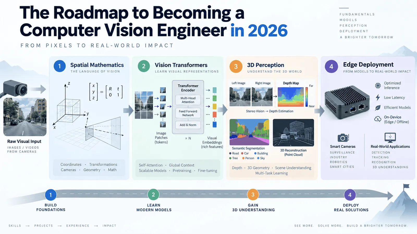
The Roadmap to Becoming a Computer Vision Engineer in 2026
A four-stage technical roadmap for becoming a computer vision engineer, from spatial mathematics and ViTs through 3D neural rendering and edge deployment optimization.
以下正文同步自 KDnuggets,版权归原站所有,已转换为易读排版。
Computer vision (CV) has moved far beyond object detection and image classification. In 2026, CV engineers work at the intersection of foundation models, spatial computing, and embedded hardware, building systems that perceive, reason over, and act on the visual world in real time.
The demand for engineers who can operate across this full stack is growing steadily. Autonomous vehicles, robotic warehouses, medical imaging platforms, and spatial computing devices all share a common need: engineers who understand not just model architecture, but the full pipeline from sensor to production inference.
This roadmap covers four stages, progressing from the spatial mathematics and foundational vision primitives that everything else depends on, through to edge deployment and hardware-aware optimization. Each stage builds directly on the previous one.
Every CV system is ultimately a system for reasoning about geometry. Before working with modern vision architectures, you need a working understanding of the mathematics that make visual reasoning possible.
The core concepts at this stage include matrix transformations, coordinate frames, projective geometry, and multi-view geometry. These aren't abstract. They determine how a camera maps a 3D world onto a 2D sensor, how two camera views can reconstruct depth, and how coordinate systems relate across sensors in a multi-camera rig.
On the implementation side, start building fluency with PyTorch for tensor manipulation, which remains the standard framework for vision research and production. Pair this with synthetic data augmentation pipelines. Albumentations is the most widely used library for this, offering fast, composable transforms that simulate lighting variation, geometric distortion, and occlusion without collecting new data.
Feature representation is the third pillar of this stage. Understand the distinction between convolutional backbones (ResNet, EfficientNet) and attention-based backbones. Contrastive representation learning — where models learn by comparing similar and dissimilar examples — has become a standard technique for learning useful embeddings before downstream fine-tuning.
Recommended resources: Multiple View Geometry in Computer Vision by Hartley and Zisserman (the canonical reference); Stanford CS231n lecture notes (free online); the PyTorch documentation's tensor tutorial series.
Portfolio exercise: Implement a basic stereo depth estimation pipeline using two calibrated images. Visualize the disparity map and document where the estimation fails and why.
The shift from convolutional neural networks (CNNs) to transformer-based architectures for vision has reshaped what CV engineers need to know. Vision Transformers (ViTs) process images as sequences of fixed-size patches, applying self-attention across those patches rather than local convolutional filters. Swin Transformers extended this with hierarchical, windowed attention that makes the approach practical for high-resolution inputs.
Beyond pure vision models, the more significant development is the emergence of vision-language models (VLMs). Models like CLIP and SigLIP learn joint embeddings across image and text modalities through contrastive training on large web-scraped datasets. The practical result is open-vocabulary understanding: you can query a visual scene with natural language descriptions rather than fixed class labels.
This unlocks a class of techniques called open-vocabulary detection. Models like OWL-ViT and Grounding DINO extend this capability to object localization, letting you detect any object described in text without retraining on labeled examples of that object.
The Segment Anything Model 2 (SAM 2) from Meta takes a different approach, offering promptable, zero-shot segmentation for both static images and video streams. A user or upstream model provides a point, bounding box, or text prompt, and SAM 2 produces a high-quality segmentation mask without task-specific training.
Understanding how these foundation models work, where they fail (domain shift, fine-grained distinctions, rare objects), and how to compose them into pipelines is the central skill of this stage.
import torch from PIL import Image import requests from transformers import AutoProcessor, AutoModelForZeroShotObjectDetection
model_id = "IDEA-Research/grounding-dino-tiny" processor = AutoProcessor.from_pretrained(model_id) model = AutoModelForZeroShotObjectDetection.from_pretrained(model_id)
image = Image.open("scene.jpg") text_prompt = "a red forklift. a safety helmet."
inputs = processor(images=image, text=text_prompt, return_tensors="pt") outputs = model(**inputs)
This runs open-vocabulary detection using a text prompt against a scene image, with no task-specific training required.
Recommended resources: An Image is Worth 16x16 Words (the original ViT paper); the Hugging Face Transformers documentation for hands-on model loading; Meta AI's SAM 2 repository and paper.
Portfolio exercise: Build a zero-shot object detection demo using Grounding DINO. Test it across three different domains (indoor scenes, outdoor scenes, a specialized domain like medical or industrial) and document where the open-vocabulary approach breaks down.
As CV systems move from image understanding to spatial reasoning, the skill set expands significantly. This stage covers the representations and algorithms that let systems understand and reconstruct the 3D world from 2D inputs.
The primary 3D representations you'll work with are point clouds, voxel grids, and signed distance fields (SDFs). Each has different memory characteristics, computational costs, and downstream application fits. Point clouds are the natural output of LiDAR sensors and structure-from-motion pipelines. Voxel grids offer regular spatial structure at the cost of memory. SDFs represent geometry as continuous functions, enabling differentiable rendering.
Depth estimation is the entry point for most 3D work. Depth Anything (v2 in particular) is the current leading monocular depth estimation model, producing relative or metric depth maps from a single RGB image without any additional sensors.
Neural rendering has developed rapidly. Neural Radiance Fields (NeRFs) learn to synthesize novel views of a scene from a set of posed images. 3D Gaussian Splatting offers a faster, more memory-efficient alternative that has largely displaced NeRFs for real-time applications, enabling interactive novel view synthesis on consumer hardware.
Spatial perception, relevant for robotics and autonomous systems, requires understanding Visual Odometry (VO) and Simultaneous Localization and Mapping (SLAM). These techniques let systems estimate their own position and build a map of their environment incrementally using only camera inputs.
import numpy as np import open3d as o3d
Load point cloud from depth map and camera intrinsics
depth = np.load("depth_map.npy") fx, fy, cx, cy = 525.0, 525.0, 319.5, 239.5
h, w = depth.shape u, v = np.meshgrid(np.arange(w), np.arange(h)) z = depth x = (u - cx) * z / fx y = (v - cy) * z / fy
points = np.stack([x, y, z], axis=-1).reshape(-1, 3) pcd = o3d.geometry.PointCloud() pcd.points = o3d.utility.Vector3dVector(points) o3d.io.write_point_cloud("output.ply", pcd)
This reconstructs a 3D point cloud from a depth map using known camera intrinsics, a technique used in depth-sensor pipelines, robotic mapping, and augmented reality (AR) applications.
Recommended resources: The Open3D documentation for 3D data processing; Structure from Motion Revisited by Schönberger and Frahm; the 3D Gaussian Splatting original paper and the nerfstudio library for neural rendering experiments.
Portfolio exercise: Use Depth Anything to generate depth maps from a short video clip. Convert the depth maps to a point cloud sequence and visualize the 3D reconstruction.
The final stage is where systems engineering meets vision. A model that performs well on a GPU workstation isn't automatically a production asset. Getting CV systems to run reliably on constrained hardware, at low latency, without unacceptable accuracy loss is a distinct and highly valued discipline.
Model compression covers three primary techniques:
Hardware execution frameworks are the next layer. TensorRT (NVIDIA) and ONNX Runtime are the standard paths for deploying optimized models to GPU and CPU targets respectively. OpenVINO (Intel) supports deployment to Intel CPUs, integrated GPUs, and vision processing units (VPUs). For embedded deployment, you'll encounter NVIDIA Jetson modules, Apple Silicon's Neural Engine, and a growing range of embedded neural processing units (NPUs) in devices like the Raspberry Pi AI Kit.
Multi-camera, high-throughput streaming introduces pipeline engineering concerns. Managing RTSP stream ingestion, synchronizing frames across cameras, batching efficiently, and maintaining throughput at 30+ FPS under load requires careful systems design. NVIDIA DeepStream is the standard toolkit for GPU-accelerated video analytics pipelines.
import tensorrt as trt import numpy as np
logger = trt.Logger(trt.Logger.WARNING) with open("model.trt", "rb") as f, trt.Runtime(logger) as runtime: engine = runtime.deserialize_cuda_engine(f.read())
context = engine.create_execution_context()
Allocate buffers and run inference
input_shape = context.get_tensor_shape("input") print(f"Engine input shape: {input_shape}")
This loads a compiled TensorRT engine and prepares it for inference, the standard pattern for deploying quantized vision models to NVIDIA hardware.
Recommended resources: The TensorRT developer guide; ONNX Runtime documentation; Hailo's edge AI developer resources; the NVIDIA Jetson getting-started guides for embedded deployment.
Portfolio exercise: Take a pretrained object detection model (YOLOv8 or RT-DETR), export it to ONNX, quantize it with TensorRT, and benchmark the accuracy and latency difference between FP32 and INT8 versions on a local GPU.
Computer vision engineering in 2026 is a layered discipline. The mathematics are foundational but not sufficient. The architectures are evolving fast but build on stable principles. The deployment constraints are real and often underestimated.
The engineers who stand out in this field are those who can move fluidly between levels of abstraction — from the geometry of a camera model, to the attention patterns of a ViT, to the instruction set of an edge accelerator. That versatility takes time to build, which is why developing it systematically, stage by stage, pays off.
Work through real projects at each stage. The skill gaps this roadmap addresses are measurable, and closing them one stage at a time is the most reliable path through.
正文由 探How 从来源站点 RSS 同步,内容未经改写;遇到排版缺失或需要图片、视频时请以原文为准。